
Personalized Recommendations at Etsy

Providing personalized recommendations is important to our online marketplace. It benefits both buyers and sellers: buyers are shown interesting products that they might not have found on their own, and products get more exposure beyond the seller’s own marketing efforts. In this post we review some of the methods we use for making recommendations at Etsy. The MapReduce implementations of all these methods are now included in our open-source machine learning package “Conjecture” which was described in a previous post.
Computing recommendations basically consists of two stages. In the first stage we build a model of users’ interests based on a matrix of historic data, for example, their past purchases or their favorite listings (those unfamiliar with matrices and linear algebra see e.g., this review). The models provide vector representations of users and items, and their inner products give an estimate of the level of interest a user will have in the item (higher values denote a greater degree of estimated interest). In the second stage, we compute recommendations by finding a set of items for each user which approximately maximizes the estimate of the interest.
The model of users and items can be also used in other ways, such as finding users with similar interests, items which are similar from a “taste” perspective, items which complement each other and could be purchased together, etc.
Matrix Factorization
The first stage in producing recommendations is to fit a model of users and items to the data. At Etsy, we deal with “implicit feedback” data where we observe only the indicators of users’ interactions with items (e.g., favorites or purchases). This is in contrast to “explicit feedback” where users give ratings (e.g. 3 of 5 stars) to items they’ve experienced. We represent this implicit feedback data as a binary matrix, the elements are ones in the case where the user liked the item (i.e., favorited it) or a zero if they did not. The zeros do not necessarily indicate that the user is not interested in that item, but only that they have not expressed an interest so far. This may be due to disinterest or indifference, or due to the user not having seen that item yet while browsing.
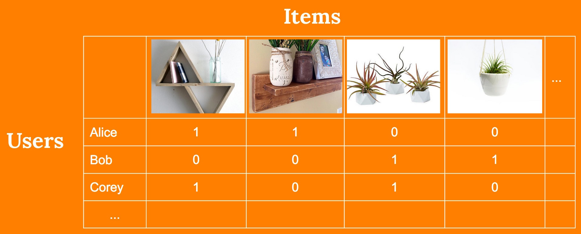 An implicit feedback dataset in which a set of users have “favorited” various items, note that we do not observe explicit dislikes, but only the presence or absence of favorites
The underpinning assumption that matrix factorization models make is that the affinity between a user and an item is explained by a low-dimensional linear model. This means that each item and user really corresponds to an unobserved real vector of some small dimension. The coordinates of the space correspond to latent features of the items (these could be things like: whether the item is clothing, whether it has chevrons, whether the background of the picture is brown etc.), the elements for the user vector describe the users preferences for these features. We may stack these vectors into matrices, one for users and one for items, then the observed data is in theory generated by taking the product of these two unknown matrices and adding noise:
 The underpinning low dimensional model from which the observed implicit feedback data is generated, "d" is the dimension of the model.
We therefore find a vector representation for each user and each item. We compute these vectors so that the inner product between a user vector and item vector will approximate the observed value in the implicit feedback matrix (i.e., it will be close to one in the case the user favorited that item and close to zero if they didn’t).
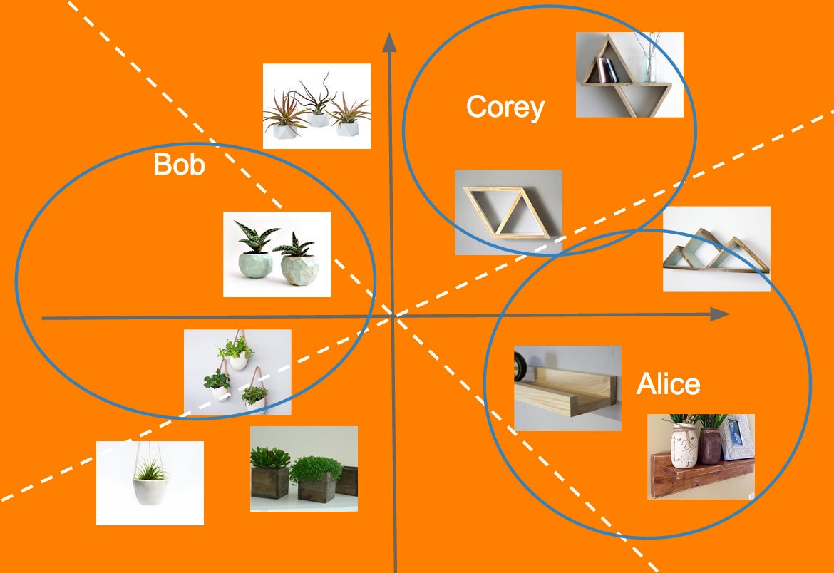
 The results of fitting a two dimensional model to the above dataset, in this small example the the first discovered features roughly corresponds to whether the item is a shelf or not, and the second to whether it is in a “geometric” style.
Since the zeros in the matrix do not necessarily indicate disinterest in the item, we don’t want to force the model to fit to them, since the user may actually be interested in some of those items. Therefore we find the decomposition which minimizes a weighted error function, where the weights for nonzero entries in the data matrix are higher than those of the zero entries. This follows a paper which suggested this method. How to set these weights depends on how sparse the matrix is, and could be found through some form of cross validation).
What happens when we optimize the weighted loss function described above, is that the reconstructed matrix (the product of the two factors) will often have positive elements where the input matrix has zeros, since we don’t force the model to fit to these as well as to the non-zeros. These are the items which the user may be interested in but has not seen yet. The reason this happens is that in order for the model to fit well, users who have shown interest in overlapping sets of items will have similar vectors, and likewise for items. Therefore the unexplored items which are liked by other users with similar interests will often have a high value in the reconstructed matrix.
Alternating Least Squares
To optimize the model, we alternate between computing item matrix and user matrix, and at each stage we minimize the weighted squared error, holding the other matrix fixed (hence the name “alternating least squares”). At each stage, we can compute the exact minimizer of the weighted square error, since an analytic solution is available. This means that each iteration is guaranteed not to increase the total error, and to decrease it unless the two matrices already constitute a local minimum of the error function. Therefore the entire procedure gradually decreases the error until a local minimum is reached. The quality of these minima can vary, so it may be a reasonable idea to repeat the procedure and select the best one, although we do not do this. A demo of this method in R is available here.
This computation lends itself very naturally to implementation in MapReduce, since e.g., when updating a vector for a user, all that is needed are the vectors for the items which he has interacted with, and the small square matrix formed by multiplying the items matrix by its own transpose. This way the computation for each user typically can be done even with limited amounts of memory available, and each user may be updated in parallel. Likewise for updating items. There are some users which favorite huge numbers of items and likewise items favorited by many users, and those computations require more memory. In these cases we can sub-sample the input matrix, either by filtering out these items, or taking only the most recent favorites for each user.
After we are satisfied with the model, we can continue to update it as we observe more information, by repeating a few steps of the alternating least squares every night, as more items, users, and favorites come online. New items and users can be folded into the model easily, so long as there are sufficiently many interactions between them and existing users and items in the model respectively. Productionizable MapReduce code for this method is available here.
Stochastic SVD
The alternating least squares described above gives us an easy way to factorize the matrix of user preferences in MapReduce. However, this technique has the disadvantage of requiring several iterations, sometimes taking a long time to converge to a quality solution. An attractive alternative is the Stochastic SVD. This is a recent method which approximates the well-known Singular Value Decomposition of a large matrix, and which admits a non iterative MapReduce implementation. We implement this as a function which can be called from any scalding Hadoop MapReduce job.
A fundamental result in linear algebra is that the matrix formed by truncating the singular value decomposition after some number of dimensions is the best approximation to that matrix (in terms of square error) among all matrices of that rank. However we note that using this method we cannot do the same “weighting” to the error as we did when optimizing via alternating least squares. Nevertheless for datasets where the zeros do not completely overwhelm the non-zeros then this method is viable. For example we use it to build a model from the favorites, whereas it fails to provide a useful model from purchases which are much more sparse, and where this weighting is necessary.
An advantage of this method is that it produces matrices with a nice orthonormal structure, which makes it easy to construct the vectors for new users on the fly (outside of a nightly recomputation of the whole model), since no matrix inversions are required. We also use this method to produce vector representations of other lists of items besides those a user favorited, for example treasuries and other user curated lists on Etsy. This way we may suggest other relevant items for those lists.
Producing Recommendations
Once we have a model of users and items we use it to build product recommendations. This is a step which seems to be mostly overlooked in the research literature. For example, we cannot hope to compute the product of the user and item matrices, and then find the best unexplored items for each user, since this requires time proportional to the product of the number of items and the number of users, both of which are in the hundreds of millions.
One research paper suggests using a tree data structure to allow for a non-exhaustive search of the space, by pruning away entire sets of items where the inner products would be too small. However we observed this method to not work well in practise, possibly due to the curse of dimensionality with the type of models we were using (with hundreds of dimensions).
Therefore we use approximate methods to compute the recommendations. The idea is to first produce a candidate set of items, then to rank them according to the inner products, and take the highest ones. There are a few ways to produce candidates, for example, the listings from favorite shops of a user, or those textually similar to his existing favorites. However the main way we use is “locality sensitive hashing” (LSH) where we divide the space of user and item vectors into several hash bins, then take the set of items which are mapped to the same bin as each user.
Locality Sensitive Hashing
Locality sensitive hashing is a technique used to find approximate nearest neighbors in large datasets. There are several variants, but we focus on one designed to handle real-valued data and to approximate the nearest neighbors in the Euclidean distance.
The idea of the method is to partition the space into a set of hash buckets, so that points which are near to each other in space are likely to fall into the same bucket. The way we do this is by constructing some number “p” of planes in the space so that they all pass through the origin. This divides the space up into 2^p convex cones, each of which constitutes a hash bucket.
Practically we implement this by representing the planes in terms of their normal vectors. The side of the plane that a point falls on is then determined by the sign of the inner product between the point and the normal vector (if the planes are random then we have non-zero inner products almost surely, however we could in principle assign those points arbitrarily to one side or the other). To generate these normal vectors we just need directions uniformly at random in space. It is well known that draws from an isotropic Gaussian distribution have this property.
We number the hash buckets so that the i^th bit of the hash-code is 1 if the inner product between a point and the i^th plane is positive, and 0 otherwise. This means that each plane is responsible for a bit of the hash code.
After we map each point to its respective hash bucket, we can compute approximate nearest neighbors, or equivalently, approximate recommendations, by examining only the vectors in the bucket. On average the number in each bucket will be 2^{-p} times the total number of points, so using more planes makes the procedure very efficient. However it also reduces the accuracy of the approximation, since it reduces the chance that nearby points to any target point will be in the same bucket. Therefore to achieve a good tradeoff between efficiency and quality, we repeat the hashing procedure multiple times, and then combine the outputs. Finally, to add more control to the computational demands of the procedure, we throw away all the hash bins which are too large to allow efficient computation of the nearest neighbors. This is implemented in Conjecture here.
Other Thoughts
Above are the basic techniques for generating personalized recommendations. Over the course of developing these recommender systems, we found a few modifications we could make to improve the quality of the recommendations.
- Normalizing the vectors before computation: As stated, the matrix factorization models tend to produce vectors with large norms for the popular items. A result is that some popular items may get recommended to many users even if they are not necessarily the most aligned with the users tastes. Therefore, before computing recommendations, we normalized all the item vectors. This also makes the use of approximate nearest neighbors theoretically sound: since when all vectors have unit norms, maximum inner products to a user vector are achieved by the nearest item vectors.
- Shop diversity: Etsy is a marketplace consisting of many sellers. So as to be fair to these sellers, we limit the number of recommendations from a single shop that we present to each user. Since users may click through to the shop anyway, exposing additional items available from this shop, this does not seem to present a problem in terms of recommendation quality.
- Item diversity: To make the recommendations more diverse, we take a candidate set of say 100 nearest neighbors to the user, then we filter those out by removing any item which is within some small distance of a higher ranked item, where the distance is measured in the Euclidean distance between the item vectors.
- Reranked Items from Similar Users: We used the LSH code to find nearest neighbors among the users (so for each user we find users with similar tastes). Then to produce item recommendations we can take those users favorite listings, and re-rank them according to the inner products between the item vectors and the target users vector. This lead to seemingly better and more relevant recommendations, although a proper experiment remains to be done.
Conclusion
In summary we described how we can build recommender systems for e-commerce based on implicit feedback data. We built a system which computes recommendations on Hadoop, which is now part of our open source machine learning package “Conjecture.” Finally we shared some additional tweaks that can be made to potentially improve the quality of recommendations.